Examples

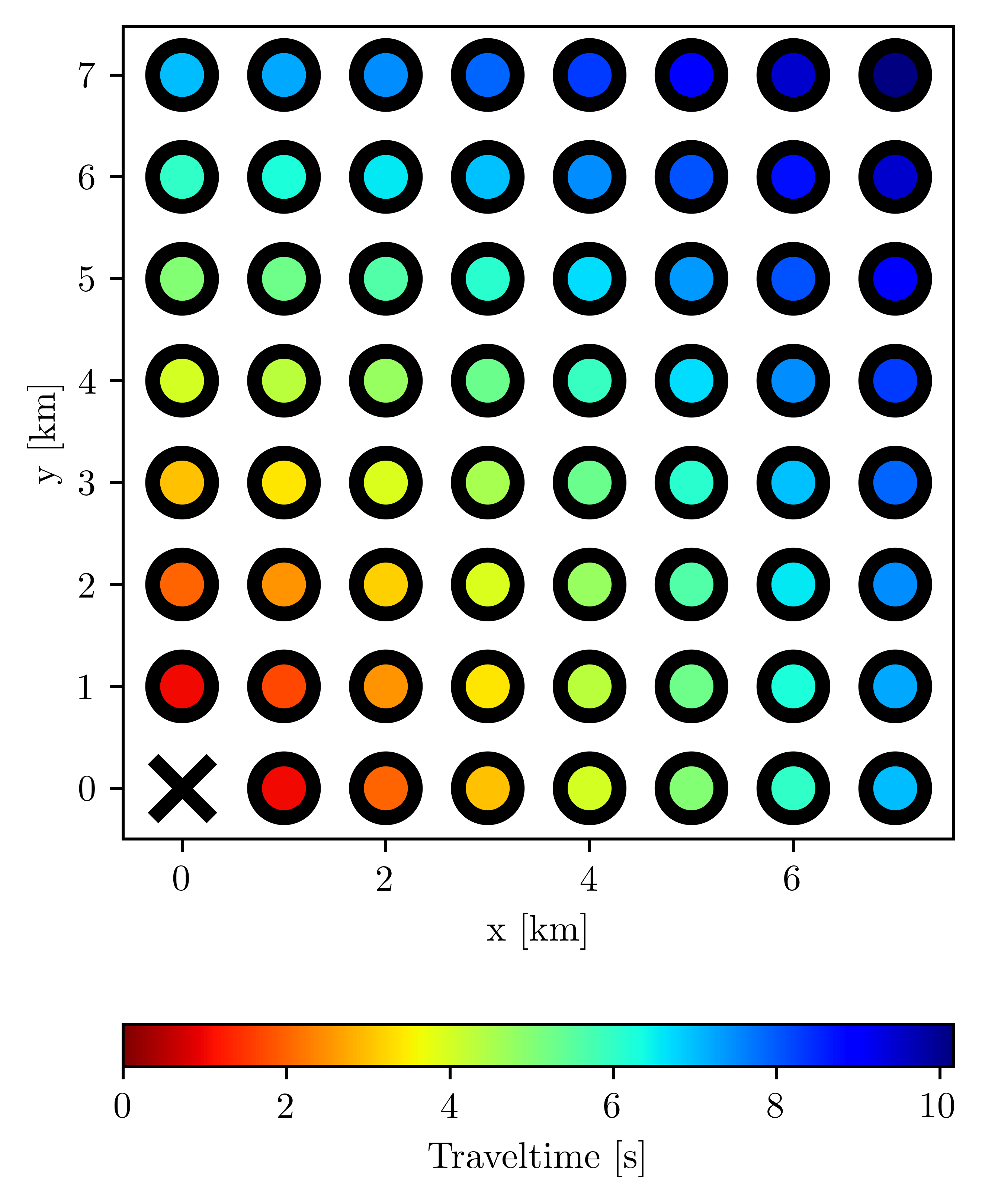
Cartesian 2D

This example demonstrates the trivial case of a point source at \((x, y) = (0, 0)\) in a homogeneous velocity model where \(v(x, y) = 1\) [km/s] using a 8 x 8 Cartesian computational grid. Note that this is really a 3D problem with only a single layer of nodes in the z direction.

# Import modules.
import numpy as np
import pykonal

# Instantiate EikonalSolver object using Cartesian coordinates.
solver = pykonal.EikonalSolver(coord_sys="cartesian")
# Set the coordinates of the lower bounds of the computational grid.
# For Cartesian coordinates this is x_min, y_min, z_min.
# In this example, the origin is the lower bound of the computation grid.
solver.velocity.min_coords = 0, 0, 0
# Set the interval between nodes of the computational grid.
# For Cartesian coordinates this is dx, dy, dz.
# In this example the nodes are separated by 1 km in in each direction.
solver.velocity.node_intervals = 1, 1, 1
# Set the number of nodes in the computational grid.
# For Cartesian coordinates this is nx, ny, nz.
# This is a 2D example, so we only want one node in the z direction.
solver.velocity.npts = 8, 8, 1
# Set the velocity model.
# In this case the velocity is equale to 1 km/s everywhere.
solver.velocity.values = np.ones(solver.velocity.npts)

# Initialize the source. This is the trickiest part of the example.
# The source coincides with the node at index (0, 0, 0)
src_idx = 0, 0, 0
# Set the traveltime at the source node to 0.
solver.traveltime.values[src_idx] = 0
# Set the unknown flag for the source node to False.
# This is an FMM state variable indicating which values are completely
# unknown. Setting it to False indicates that the node has a tentative value
# assigned to it. In this case, the tentative value happens to be the true,
# final value.
solver.unknown[src_idx] = False
# Push the index of the source node onto the narrow-band heap.
solver.trial.push(*src_idx)

# Solve the system.
solver.solve()

# And finally, get the traveltime values.
print(solver.traveltime.values)

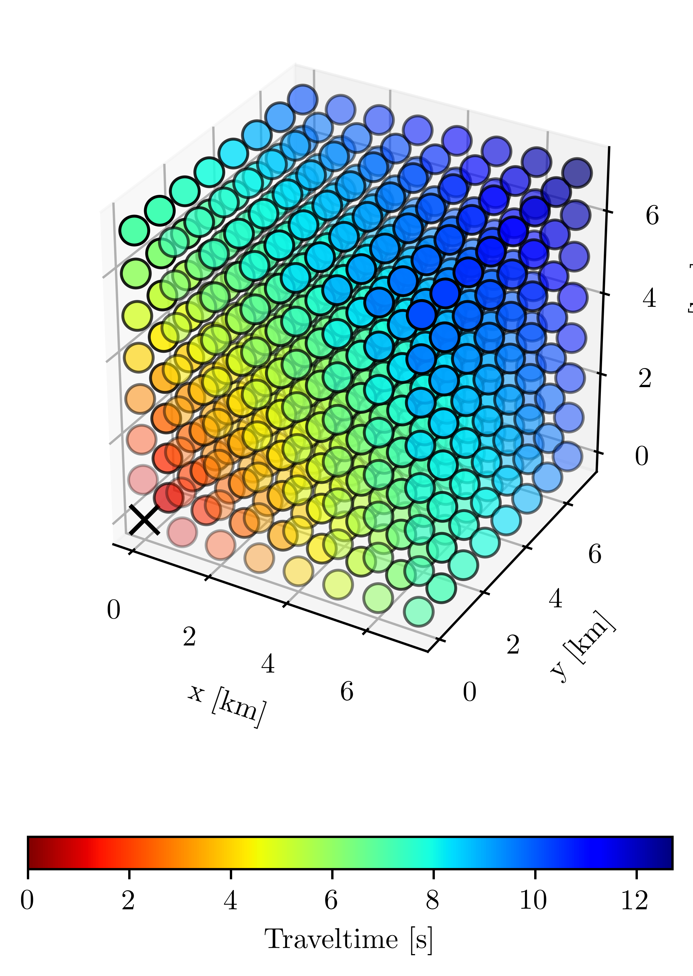
Cartesian 3D

Identical to the Cartesian 2D example except this time extend the computational grid by 8 nodes in the z direction.

import numpy as np
import pykonal

# Initialize the solver.
solver = pykonal.EikonalSolver(coord_sys="cartesian")
solver.velocity.min_coords = 0, 0, 0
solver.velocity.node_intervals = 1, 1, 1
# This time we want a 3D computational grid, so set the number of grid nodes
# in the z direction to 8 as well.
solver.velocity.npts = 8, 8, 8
solver.velocity.values = np.ones(solver.velocity.npts)

# Initialize the source.
src_idx = 0, 0, 0
solver.traveltime.values[src_idx] = 0
solver.unknown[src_idx] = False
solver.trial.push(*src_idx)

# Solve the system.
solver.solve()

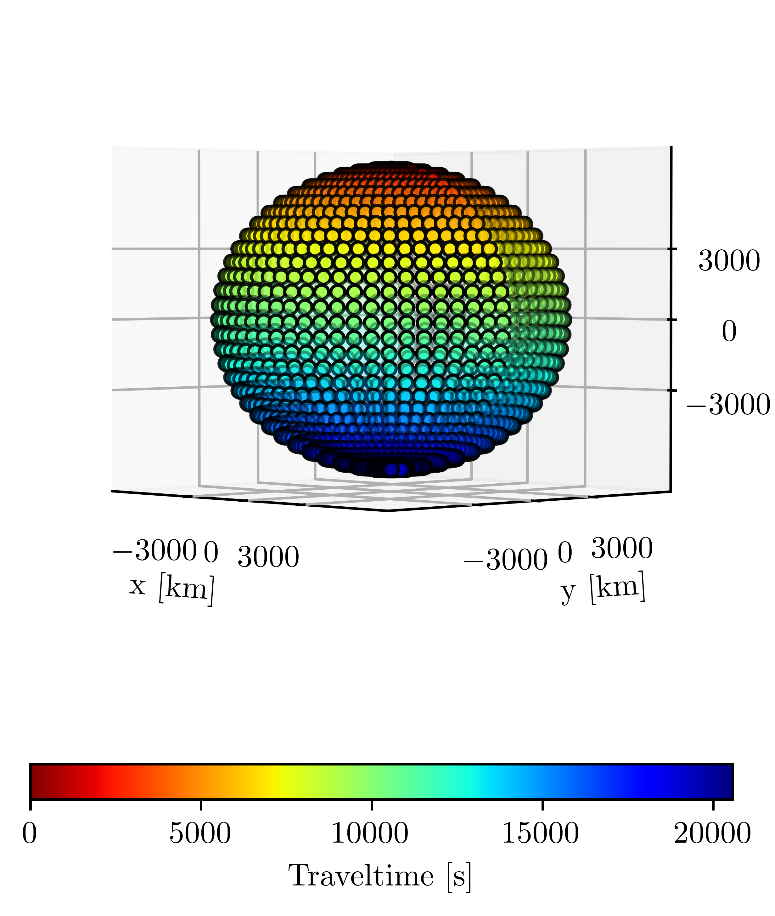
Spherical 2D (Spherical shell)

This example demonstrates the trivial case of a point source at the North pole \((\rho, \theta, \phi) = (6371, 0, 0)\) in a homogeneous velocity model where \(v(\rho, \theta, \phi) = 1\) [km/s] using a 1 x 33 x 64 spherical-shell computational grid. This example demonstrates how to use PyKonal to track surface waves.

import numpy as np
import pykonal

solver = pykonal.EikonalSolver(coord_sys="spherical")
solver.velocity.min_coords = 6371., 0, 0
solver.velocity.node_intervals = 1, np.pi/32, np.pi/32
solver.velocity.npts = 1, 33, 64
solver.velocity.values = np.ones(solver.velocity.npts)

src_idx = (0, 0, 0)
solver.traveltime.values[src_idx] = 0
solver.unknown[src_idx] = False
solver.trial.push(*src_idx)
solver.solve()