Spherical 2D (Spherical shell)
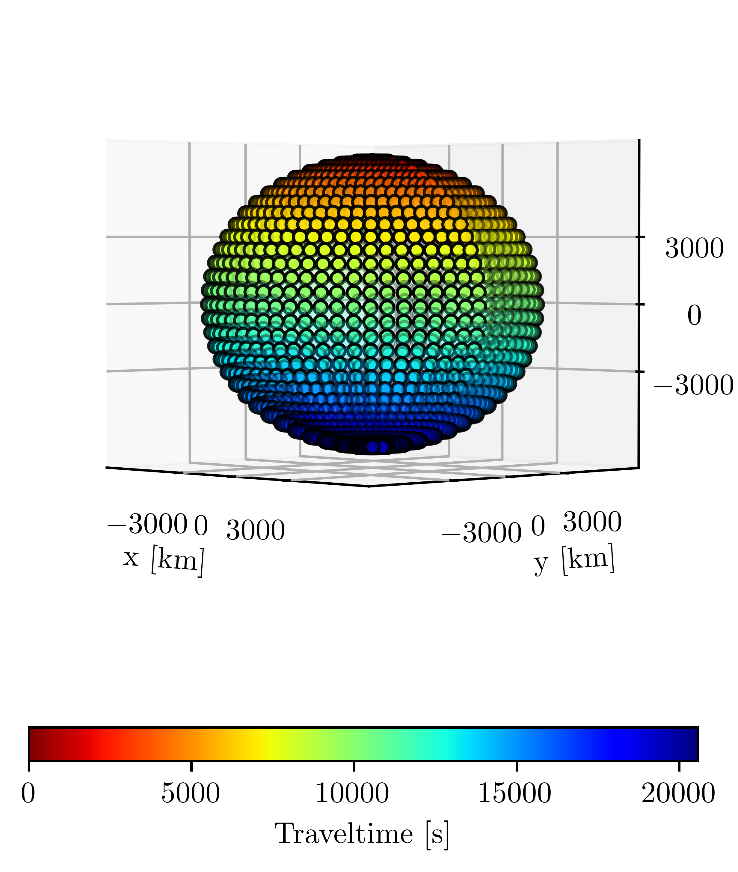
This example demonstrates the trivial case of a point source at the North pole \((\rho, \theta, \phi) = (6371, 0, 0)\) in a homogeneous velocity model where \(v(\rho, \theta, \phi) = 1\) [km/s] using a 1 x 33 x 64 spherical-shell computational grid. This example demonstrates how to use PyKonal to track surface waves.
import numpy as np
import pykonal

solver = pykonal.EikonalSolver(coord_sys="spherical")
solver.velocity.min_coords = 6371., 0, 0
solver.velocity.node_intervals = 1, np.pi/32, np.pi/32
solver.velocity.npts = 1, 33, 64
solver.velocity.values = np.ones(solver.velocity.npts)

src_idx = (0, 0, 0)
solver.traveltime.values[src_idx] = 0
solver.unknown[src_idx] = False
solver.trial.push(*src_idx)
solver.solve()